AASTK documentation
Documentation for the amino acid sequence toolkit (AASTK) version 0.1.0.
Table of contents
- AASTK synopsis
- Installation instructions
- Protein alignment score ratio (PASR)
- Clustering alignment score matrix (CASM)
- Colocated unidirectional gene organization (CUGO)
- Metadata retrieval (Meta)
- Database utilities
AASTK synopsis
The amino acid sequence toolkit (AASTK) is a suite of tools that enables construction and analyses of protein sequence datasets from the GlobDB genomes. The GlobDB is the most comprehensive resource of species-representative genomes of Bacteria and Archaea. AASTK is designed to leverage the GlobDB to create and analyse protein sequence datasets of maximum phylogenetic diversity for evolutionary and functional studies.
For some functions, AASTK uses a precomputed SQL database that includes the protein sequences of all GlobDB genomes, their genomic context, functional annotations from KEGG, COG, and PFAM, and metadata on the genomes and the protein sequences. This SQL database is available for download under Downloads. To reduce download burden, a protein fasta file containing all GlobDB amino acid sequences can be exported from the SQL database (see database utilities).
AASTK currently consists of four tools:pasr - Creating and updating comprehensive datasets of proteins of interest.casm - Clustering datasets of complex functionally diverse protein superfamilies.cugo - Assessing consensus genomic context of a protein dataset.meta - Retrieving metadata such as taxonomy, environment, and annotations from the AASTK SQL database
A short description of the main tools of AASTK can be found below. A full description of all command line tools and arguments is available on their respective pages, accessible via the dropdown menu or the links below.
Source code for AASTK is available on github.
Installation instructions
We recommend installation using conda.conda create aastkconda activate aastkconda install -c bioconda aastk
Installation instructions from source or using pip are available on github.
For AASTK to work fully, you'll need the AASTK SQL database. (WARNING: this is a 310 Gb file)
This database can be downloaded and unzipped using:wget https://fileshare.lisc.univie.ac.at/globdb/globdb_r226/globdb_r226_aastk.db.gzgunzip globdb_r226_aastk.db.gz
Then, it is useful to have a single file containing all GlobDB proteins. This can be exported from the AASTK SQL database.
To export the GlobDB proteins from the AASTK SQL database, run:aastk export_fasta -d globdb_r226_aastk.db -n 4 -o protein_fasta_dir
Protein alignment score ratio (PASR)
PASR synopsis
PASR is intended for the creation of comprehensive sequence datasets of homologous proteins by aligning all sequences in a query dataset to a (small) seed dataset of sequences of interest using DIAMOND. Thus, the query file is the large dataset containing all proteins to be searched, and the seed is the (preliminary) dataset of homologous proteins to be found in the query data.
The helper tool pasr_select can be used to select sequences to include in the final dataset, based on the PASR plot.
The PASR workflow consists of the following steps:
- Creating of a DIAMOND database of the seed dataset.
- Alignment of all sequences in the query dataset against the seed database
- Extraction of all hits from the query dataset
- Calculation of the maximum alignment score of each hit.
- Calculation of the alignment score ratio.
- Generating the PASR plot.
The entire workflow can be run using aastk pasr, as shown in the usage example below. All command line options for PASR are available on the PASR command line reference page.
Individual steps of the PASR workflow are accessible from the command line using the build, search, get_hit_seqs, max_score, bsr, and pasr_plot commands. The command line options for these 6 commands are also available on the PASR command line reference page.
PASR usage example
Basic usage:aastk pasr -m BLOSUM45 -q query.fasta -s seed.fasta -o output_dir
Where-m specifies the scoring matrix to be used, can be BLOSUM62 or BLOSUM45-q specifies the query dataset in fasta format-s specifies the seed database of homologous proteins, in fasta format-o specifies the output directory
Full command line reference for PASR.
PASR output overview
The PASR output consists of the following files:<seed_basename>_bsr.png
The PASR plot (see example below)<seed_basename>_bsr.tsv
Tab delimited file containing the plot data<seed_basename>_matched.faa
Sequences of matches in the query dataset
When PASR is run with --keep the following additional files will be kept<seed_basename>_columns.json
Column names for the bsr table<seed_basename>.dmnd
DIAMOND database of the seed sequence(s)<seed_basename>_hits.txt
DIAMOND output in tabular format<seed_basename>_matched.stats
Basic stats of the matching sequences<seed_basename>_max_scores.tsv
Maximum alignment scores of the matchesaastk subprocess stderr log
Log of the subprocesses run during pasr
The PASR plot is a scatterplot showing all matching sequences from the query dataset where the x-axis is the maximum alignment score, and the y-axis is the score against the seed database. The points are colored by identify of the hit. The histograms on each axis indicated the number of matches, to mitigate plot overcrowding.
When pasr is run with --update or when the plot is generated using pasr_select dashed lines will indicate the selected cutoff values used.
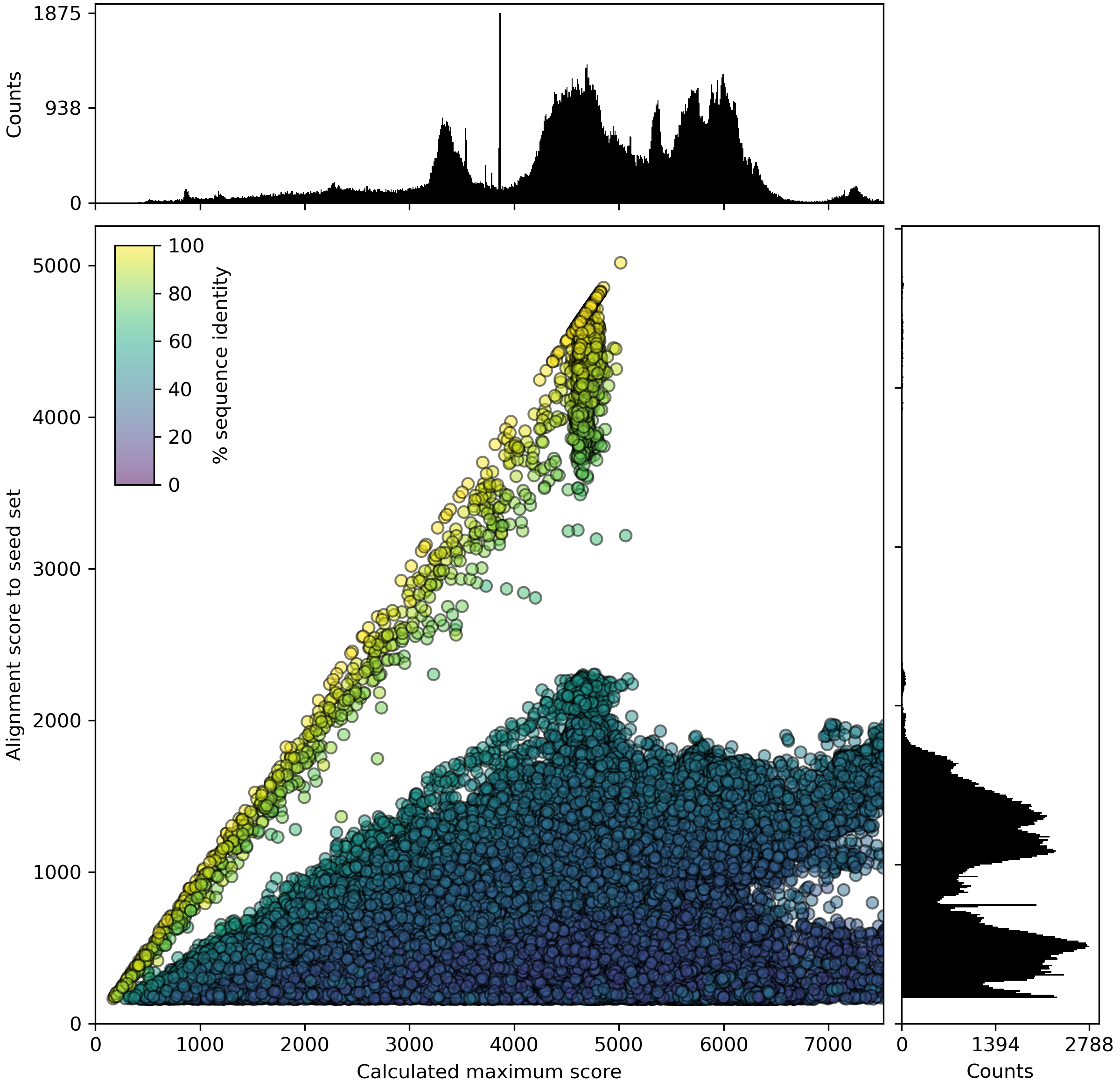
Figure 1. Example PASR plot
PASR plot of the catalytic, molybdenum containing subunit of an enzyme in the MopB superfamily. Each dot indicates a protein sequence, with the x-axis representing the calculated maximum alignment score, and the y-axis the alignment score against the seed dataset. Color of the dots represents sequence identity of the best hit in the seed dataset. Dots on the 1:1 line represent sequences already present in the seed dataset. Full length sequences (for this dataset) have a calculated maximum score (x-axis) of approx. 4500-5000. Dots with lower values on the x-axis represent partial sequences, either pseudogenes or (more commonly) sequences encoded at the edge of contigs in fragmented genomes. The x-axis is cut off at 150% of the maximum value of the y-axis
Clustering alignment score matrix (CASM)
CASM synopsis
CASM is designed to investigate the structure of a dataset of homologous proteins, such as a protein superfamily. Many protein (super)families contain members with distinct biochemical or physiological functions. Understanding the structure of a protein (super)family is an essential first step in understanding the functional landscape of a protein (super)family. Existing approaches such as phylogenetic analyses or sequence similarity networks (see for example Atkinson et al. 2009) don't scale well to the size of modern datasets.
CASM clusters sequences by generating an N x n alignment score matrix, by aligning all N sequences in a dataset against a subset of n sequences. T-distributed stochastic neighbourhood embedding (t-SNE) is then used to reduce this matrix to from n to 2 dimensions. Clusters are called using DBSCAN, and the t-SNE results can be annotated with metadata and visualised.
The helper tool casm_select can be used to select sequence clusters for further analysis.
The CASM workflow consists of the following steps:
- If no subset is provided, randomly selecting a subset of
nsequences from the dataset. - Creating a DIAMOND database of the sequence subset.
- Aligning all
Nsequences in the dataset to thensequences in the subset - Generating a (sparse) alignment score matrix with dimensions
Nxn. - Initial dimensionality reduction of the matrix with exaggerated attraction using opentSNE.
- Halting the t-SNE, and clustering the intermediate result with DBSCAN.
- Finalising the t-SNE run.
- Generating the CASM plot labeled with metadata of choice.
The entire workflow can be run using aastk casm, as shown in the usage examples below. All command line options for CASM are available on the CASM command line reference page.
Individual steps of the CASM workflow are accessible from the command line using the matrix, cluster, and casm_plot commands. The command line options for these 3 commands are also available on the CASM command line reference page.
CASM usage example
Basic command:aastk casm --fasta input.faa -o output_directory --subset_size 1000 -n 4 -p 1000
where:--fasta and -o control the input and output, --subset_size determines the number of randomly selected proteins in the subset,-n specifies the number of threads to use,-p is the t-SNE perplexiity
Full command line reference for CASM.
CASM output overview
The CASM output consists of the following files:<input fasta basename>_align_tsne_early_clusters.png
Scatterplot based on tSNE coordinates after early exaggeration, when clustering is done.<input fasta basename>_align_tsne_final_clusters.png
Scatterplot with final tSNE coordinates<input fasta basename>_align_tsne_early_clust.tsv
Tab delimited file containing the early tSNE coordinates and selected metadata for the input sequences<input fasta basename>_align_tsne_final_clust.tsv
Tab delimited file containing the final tSNE coordinates and selected metadata for the input sequences
When CASM is run with --keep the following additional files will be kept<input fasta basename>_align_matrix_metadata.json
json file storing the identifiers of the input sequences<input fasta basename>_align_matrix.npy
numpy matrix of alignment score matrix that is used for dimensionality reduction with tSNE<input fasta basename>_subsample.faa
Fasta file with the sequences of the randomly selected subsetaastk subprocess stderr log
Log of the subprocesses run during pasr
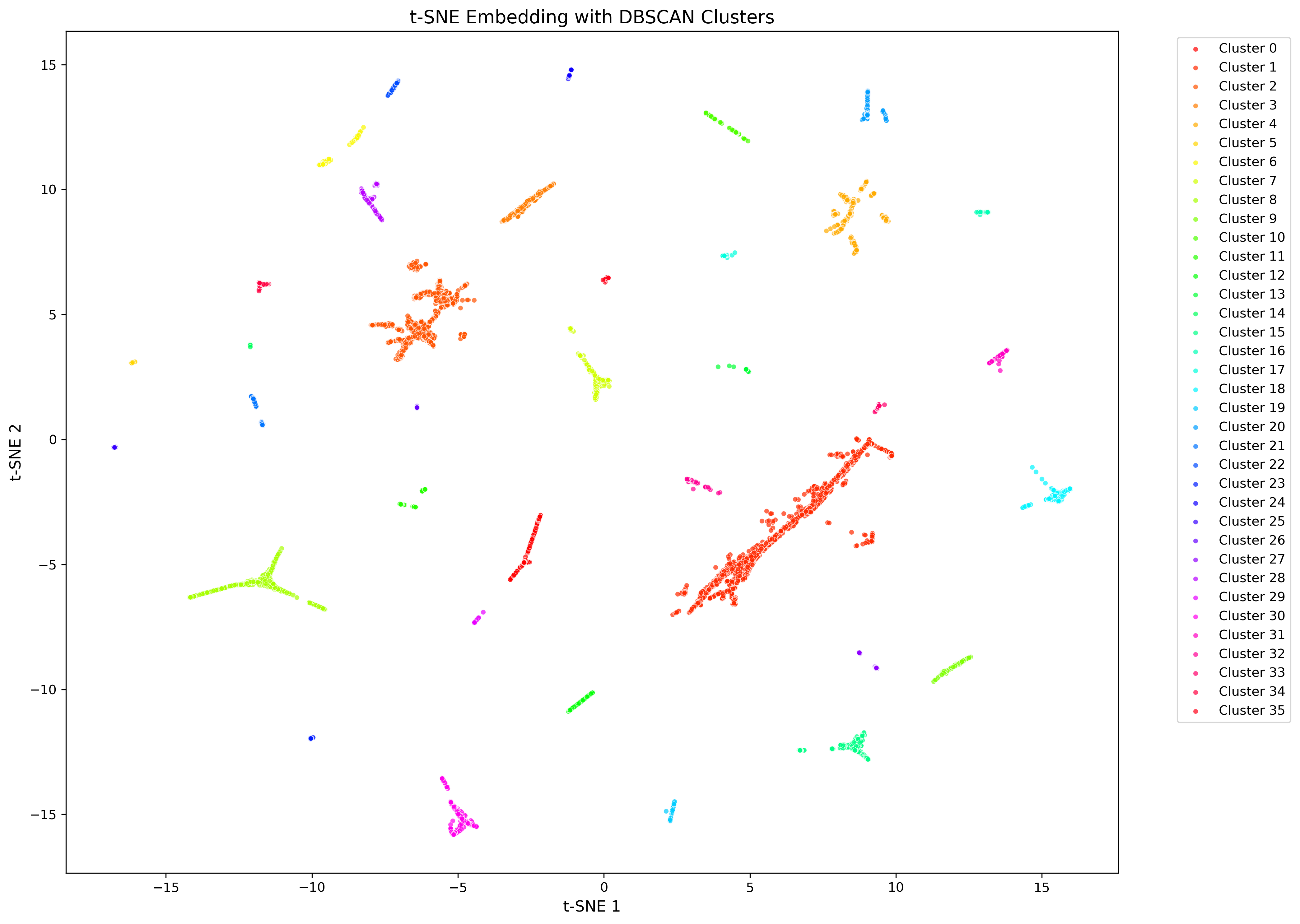
Figure 2. Example CASM plot after early exaggeration phase.
tSNE plot showing 166,445 sequences of the mopB superfamily after early exaggeration, when the clustering with DBSCAN is done. Points are colored by cluster affiliation.
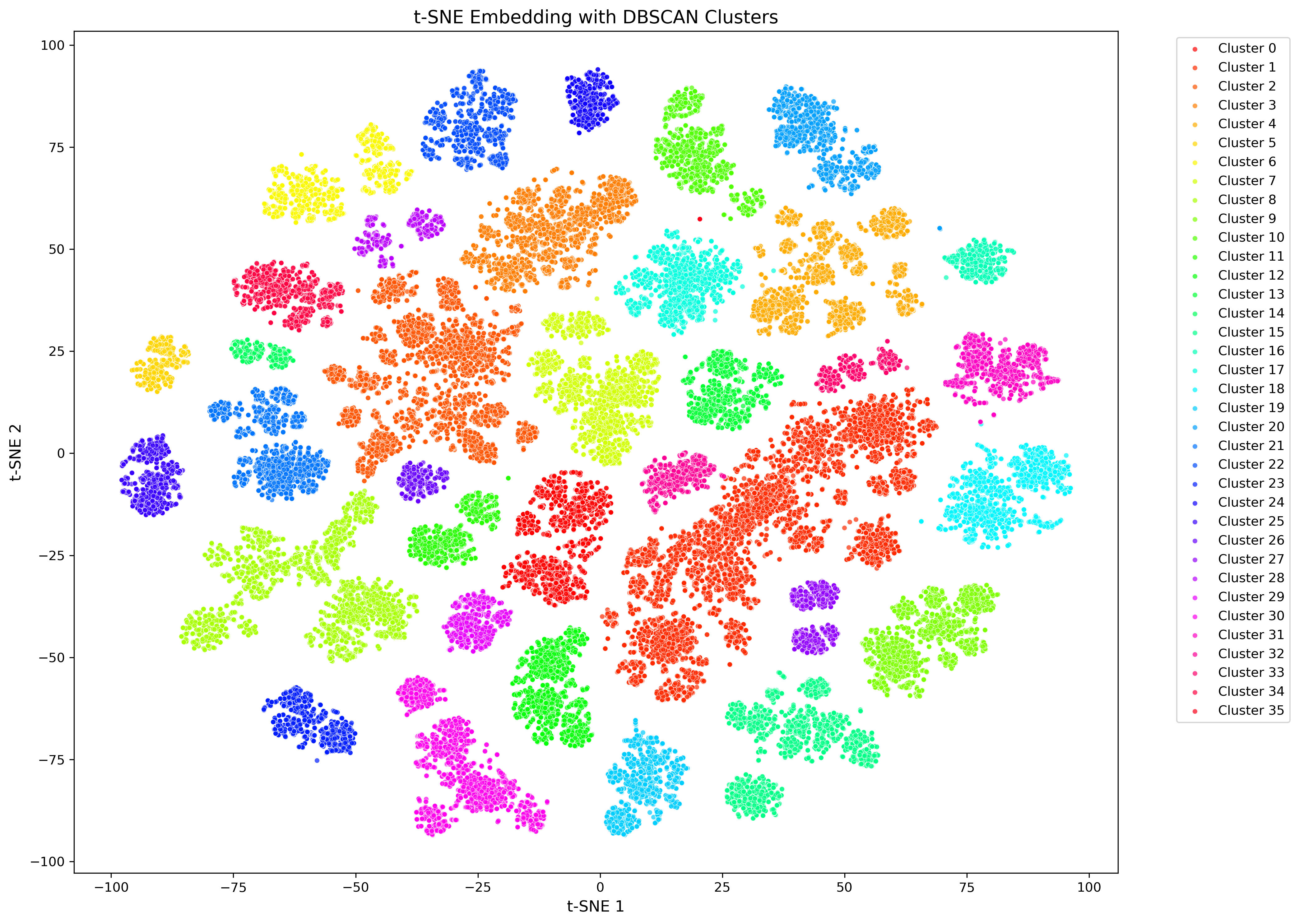
Figure 3. Example of final CASM plot
Final tSNE plot showing 166,445 sequences of the mopB superfamily. Points are colored by cluster affiliation, but can also be colored by information from the AASTK SQL database, including taxonomy, environment or culture availability.
Colocated unidirectional gene organisation (CUGO)
CUGO synopsis
CUGO is intended to retrieve and visualise the consensus genomic context of a dataset of homologous proteins. To do so, it uses information from the AASTK SQL database of the proteins in the GlobDB genomes. Each GlobDB genome is partitioned into CUGO units, that are limited by a strand change of encoded proteins, or when a contig ends. For each sequence in the input file, aastk cugo determines it's CUGO unit, and then extracts all sequences belonging to this CUGO unit, and optionally adjacent CUGO units. The sequences extracted this way are then used for visualisation.
Consensus genomic context is visualised in three plots combined into one overview figure. The first plot shows the three most common annotations per genomic position, the second the density of amino acid sequence length per position, and the third the density of number of transmembrane helices per position (see figure below). This design ensures that there is no upper limit to the size of the query dataset size from a visualisation perspective, although data retrieval time scales with query size. CUGO uses the AASTK SQL database, which as of release 226 is 318 Gb.
The helper tool cugo_select can be used to select a genomic position and export sequences for further analysis.
The CUGO workflow consists of the following steps:
- Getting the protein identifiers from the input file
- From the SQL database, identifying genes in the specified cugo range of selected identifiers
- Extracting annotation, length, and number of transmembrane helices of all identified genes
- Summarizing these data per genomic position relative to the input sequences
- Plot the summarized data as histogram or density
The entire workflow can be run using aastk cugo, as shown in the usage example below. All command line options for CUGO are available on the CUGO command line reference page.
Individual steps of the CUGO workflow are accessible from the command line using the context and cugo_plot commands. The command line options for these 2 commands are also available on the CUGO command line reference page.
CUGO usage example
aastk cugo -r 0 -l -3 -u 6 -d aastk_sql_database.db -f fasta_file.faa -o cugo_output_dir
where:-r is the range of CUGO units to be considered-l specifies the number of positions upstream of the gene of interest-u specifies the number of positions downstream of the gene of interest-d is the path to the AASTK SQL database-f and -o control the input and output
Full command line reference for CUGO.
CUGO output overview
The CUGO output consists of the following files:<input fasta basename>_context.tsv
Tab-delimited file will data on all genes making up the neighbourhood of the target genes<input fasta basename>_cugo.png
Genomic context plot showing consensus annotation, length, and transmembrane segments per position.
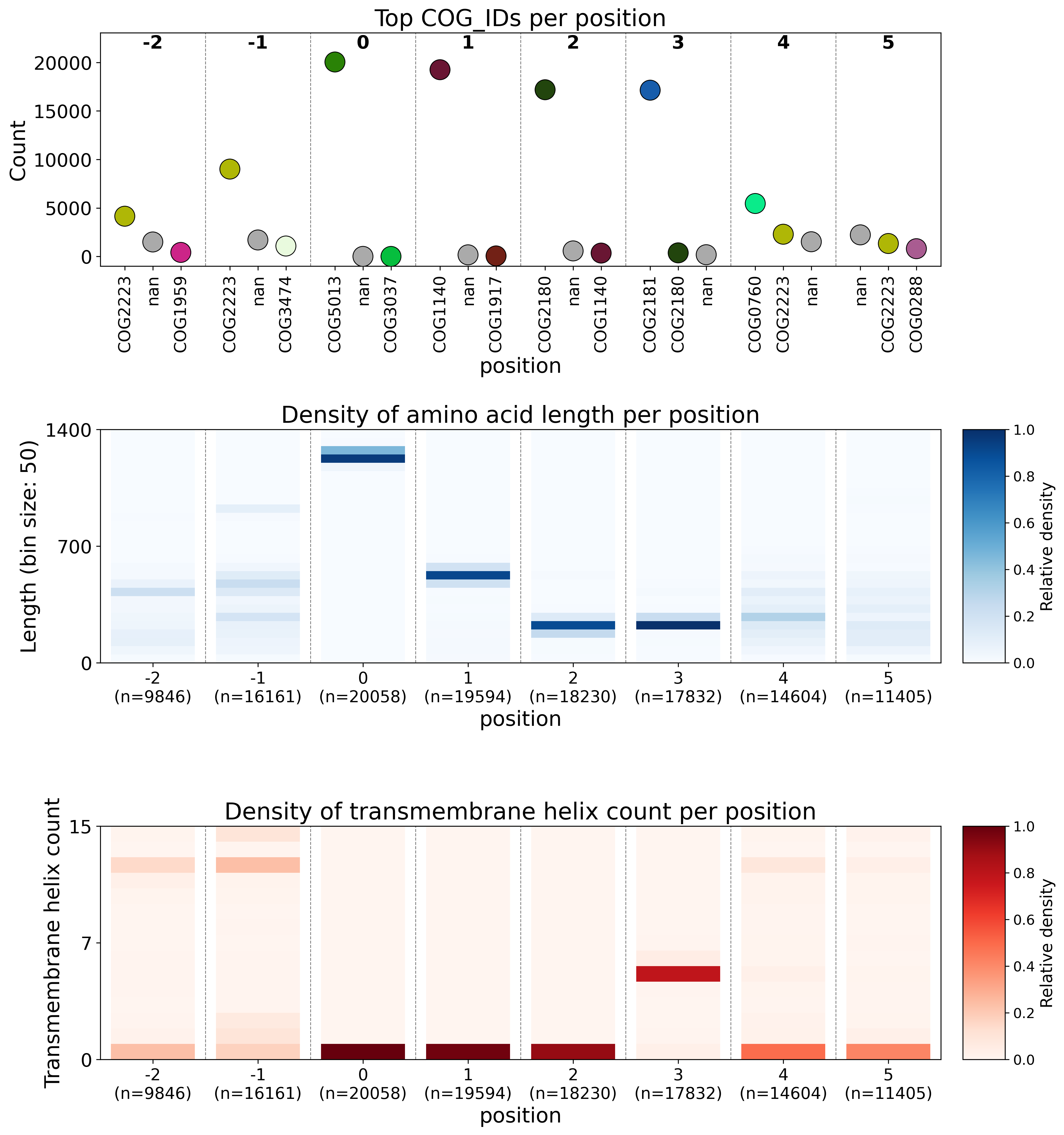
Figure 4. Example CUGO plot
The CUGO visualisation consists of three plots. The first plot shows the three most prevalent annotations per position, using a histogram like graph. Colors for each COG are consistent within and across plots. The second plot shows the number of proteins in length bins (default 50 amino acids) position, showing whether proteins at a position are conserved in an annotation independent way. The third plot shows the predicted transmembrane helices at each position.
Metadata retrieval (Meta)
Meta synopsis
Meta allows for retrieval of sequence metadata from the AASTK SQL database based on a protein fasta file or a list of protein identifiers. There are two types of metadata in the SQL database, those linked to protein sequences directly, and those linked to the genomes encoding the protein sequences. Available metadata categories are annotation (protein linked), taxonomy, culture collection availability, and two levels of environmental metadata (all genome linked). The selected metadata are written to a tsv file. A full overview of available metadata can be viewed by running aastk metadata_categories.
Meta usage example
aastk meta --all_metadata -d aastk_sql_database.db -f fasta_file.faa -o output_directory
Where:--all_metadata controls which metadata is added to the output tsv file-d is the path to the AASTK SQL database-f and -o control the input and output
Full command line reference for Meta.
Meta output overview
The meta output consists of the following files:<input fasta basename>_metadata.tsv
Tab delimited file containing the sequence IDs and selected metadata columns
Database utilities
The AASTK SQL database is constructed from a fasta file containing all GlobDB proteins sequences, and is augmented with metadata for both the genomes encoding the proteins, as well as the proteins themselves (see above and the meta command line reference for details). The database is constructed using aastk database, and checked using aastk database_check. Protein fasta files can be exported from the SQL database using aastk export_fasta.
We strongly recommend using AASTK with the provided SQL database. aastk database can take tab delimited (tsv) files for genome metadata, and requires directories with one file per genome for the protein metadata.
Full command line reference for database utilities.
How to cite
There is no publication describing AASTK yet, so for now please cite the Github repository when you use AASTK.
In addition, several parts of the software were developed independently and should be credited.
- If you use AASTK with the GlobDB protein dataset, please cite:
Speth et al. (2025) GlobDB: a comprehensive species-dereplicated microbial genome resource
https://doi.org/10.1093/bioadv/vbaf280 - If you use
aastk pasr, please cite:
Speth and Orphan (2018) Metabolic marker gene mining provides insight in global mcrA diversity and, coupled with targeted genome reconstruction, sheds further light on metabolic potential of the Methanomassiliicoccales
https://doi.org/10.7717/peerj.5614 - The environmental data from
aastk metais derived from the MetaCoOc software. A manuscript is in preparation, but in the meantime please cite:
https://github.com/bcoltman/metacooc